Using Regions of interest (ROIs) in DeepOF - Explore spatial information

What we’ll cover:

• Create a project with ROIs

• Vasic ROI functionality

• Visualize information contained in specific ROIs

• Extract information based on different ROIs

# # If using Google colab, uncomment and run this cell and the one below to set up the environment
# # Note: because of how colab handles the installation of local packages, this cell will kill your runtime.
# # This is not an error! Just continue with the cells below.
# import os
# !git clone -q https://github.com/mlfpm/deepof.git
# !pip install -q -e deepof --progress-bar off
# os.chdir("deepof")
# !curl --output tutorial_files.zip https://datashare.mpcdf.mpg.de/s/Hu1XjZkY9zml0mm/download
# !unzip tutorial_files.zip

# import os
# os.chdir("deepof")
# import os, warnings
# warnings.filterwarnings('ignore')

As usual, we import some packages and plotting gear. We’ll use python’s os library to handle paths, pickle to load saved objects, and the data entry API within DeepOF, located in deepof.data

# Import basic stuff
import os
import pickle
import deepof.data
# import plotting gear
import deepof.visuals
import matplotlib.pyplot as plt
import seaborn as sns

Creating a project with ROIs

All we have to do in the project definition to create a project with ROIs is to set the input argument “number_of_rois” to any number between 1 and 20. This will then let us draw our ROIs during project creation

my_deepof_project_raw = deepof.data.Project(
    project_path=os.path.join("tutorial_files"),
    video_path=os.path.join("tutorial_files/Videos/"),
    table_path=os.path.join("tutorial_files/Tables/"),
    project_name="deepof_tutorial_project",
    arena="circular-autodetect",
    animal_ids=["B", "W"],
    table_format="h5",
    video_format=".mp4",
    exclude_bodyparts=["Tail_1", "Tail_2", "Tail_tip"],
    video_scale="380 mm",
    iterative_imputation="partial",  # "full",
    smooth_alpha=1,
    exp_conditions="./tutorial_files/tutorial_exp_conditions.csv", # path to exp conditions table
    number_of_rois=3, # an optional input argument that allows you to draw up to 20 different regions of interest (ROI)s during project creation
)

Info! Set arena dimension to 380.0 mm!

The sampling rate of some of your videos differ. The maximum difference is 20191204_Day2_SI_JB08_Test_54: 24.99 fps and 20191204_Day2_SI_JB08_Test_63: 24.994 fps! Proceed with cauthion

As we run our Tutorial scripts automatically for testing purposes and the create function opens a GUI which would interfere with that, the follwoing line of code it is commented out. To create your own project, you can simply remove the “#” at the front of the line and execute it.

# my_deepof_project_with_rois = my_deepof_project_raw.create(force=True)

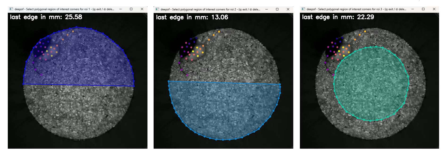
After the arenas are detected (which will take a short while with the automatic detection) one after another, three windows will plop up for you to click your three ROIs just as you would click a nanual polygonal arena (see Figure below). You will always have to click all of the ROIs for one video, then all ROIs for the next one and so on. And just as you can do with the arenas in manual mode, you can propagate single ROIs with the “p”-key. This means that the respective ROI will get copied for all following videos and you will not have to click it manually. However, this means that the ROI will be copied exactly from the previous video. If you have a ROI that may differ from video to video or if your videos are rather inconsistent, it may make more sense to manually click your ROIs for all videos. For this example case we click an upper half area, a lower half area and a central circular area (as in the Figure below).

Loading a previously initiated project

You can now continue to use your own project or just load the larger deepof test project with 53 videos.

# Load a previously saved project
my_deepof_project_with_rois = deepof.data.load_project("./tutorial_files/tutorial_project")

NOTE to better show how DeepOF deals with statistics, all results shown in the documentation version of this tutorial were obtained using the full SI dataset, containing a total of 53 animals. If you’d like to gain access to this dataset, check out the code availability statement of the main DeepOF paper.

Basic ROI functionality

For starters, let us have a look at our ROIs for our different experiment conditions. Setting a ROI number in plot_heatmaps will lead to this ROI getting applied to all experiments in the project. If a mouse is inside or outside of a ROI is determined via the position of the center of the mouse. And which mice are relevant for that evaluation is dermined via animals_in_roi.

For this example with roi_number=1 and animals_in_roi=”B” we consider all instances during which mouse B (the black mouse) was inside of ROI 1 (the upper half of the arena) for nonstressed and stressed mice. The Respectively, the position of the white mouse does not matter here.

sns.set_context("notebook")

fig, (ax1, ax2) = plt.subplots(1, 2, figsize=(12, 6))

# Nose based plot
deepof.visuals.plot_heatmaps(
    my_deepof_project_with_rois,
    ["B_Center"],
    center="arena",
    exp_condition="CSDS",
    condition_value="Nonstressed",
    ax=ax1,
    show=False,
    display_arena=True,
    experiment_id="average",
    # Time binning info
    bin_index=2,
    bin_size=60,
    samples_max=250, # we reduce the maximum number of samples per experiment to allow for a fatser function execution
    # ROI arguments
    roi_number=1,
    animals_in_roi="B",
)

# Center based plot
deepof.visuals.plot_heatmaps(
    my_deepof_project_with_rois,
    ["B_Center"],
    center="arena",
    exp_condition="CSDS",
    condition_value="Stressed",
    ax=ax2,
    show=False,
    display_arena=True,
    experiment_id="average",
    # Time binning info
    bin_index=2,
    bin_size=60,
    samples_max=250,
    # ROI arguments
    roi_number=1,
    animals_in_roi="B",
)

plt.tight_layout()
plt.show()

Info! Selected range exceeds 250 samples and has been downsampled by a factor of approx. 5
To avoid this, increase 'samples_max'. This will also result in increased computation time

Info! Selected range exceeds 250 samples and has been downsampled by a factor of approx. 5
To avoid this, increase 'samples_max'. This will also result in increased computation time

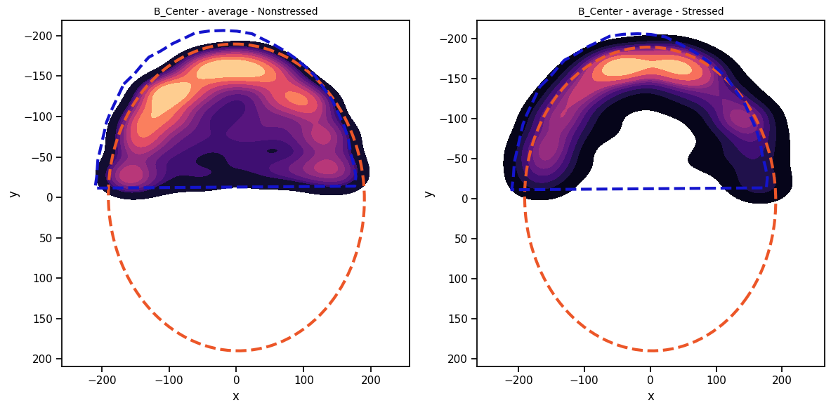
As we can see, the average of our ROIs is a bit to the left of the average arena. This is what can happen if the ROIs are not all clicked individually for all videos as the arena itself is not at the exact same position in each video.

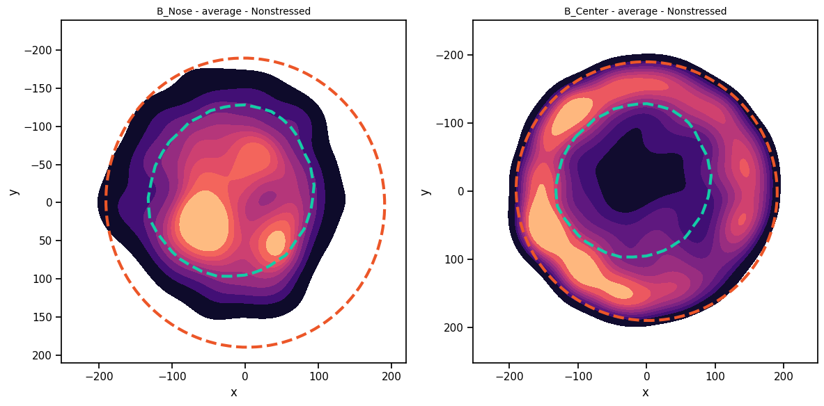
Next, just to understand the ROI funtionality a bit better, we will have a look at two special cases:

• In the first case we extract the nose positions of the black mouse whilst this black mouse was inside of ROI 3. As we can see, some activity is detected outside of the ROI. This happens because the center position of the mouse is used to determine if the mouse is inside of the ROI. Hence, a Mouse standing just on the edge of a ROI and looking outside is still technically “inside” of that ROI.

• In the second example we track the center of the black mouse for all frames during which the white mouse is inside of ROI 3. As this doesn’t apply any restrictions to the position of the black mosue, we will see activity in the whole arena.

sns.set_context("notebook")

fig, (ax1, ax2) = plt.subplots(1, 2, figsize=(12, 6))

# Nose based plot
deepof.visuals.plot_heatmaps(
    my_deepof_project_with_rois,
    ["B_Nose"],
    center="arena",
    exp_condition="CSDS",
    condition_value="Nonstressed",
    ax=ax1,
    show=False,
    display_arena=True,
    experiment_id="average",
    # Time binning info
    bin_index=2,
    bin_size=60,
    samples_max=250,
    # ROI arguments
    roi_number=3,
    animals_in_roi="B",
)

# Center based plot
deepof.visuals.plot_heatmaps(
    my_deepof_project_with_rois,
    ["B_Center"],
    center="arena",
    exp_condition="CSDS",
    condition_value="Nonstressed",
    ax=ax2,
    show=False,
    display_arena=True,
    experiment_id="average",
    # Time binning info
    bin_index=2,
    bin_size=60,
    samples_max=250,
    # ROI arguments
    roi_number=3,
    animals_in_roi="W",
)

plt.tight_layout()
plt.show()

Info! Selected range exceeds 250 samples and has been downsampled by a factor of approx. 5
To avoid this, increase 'samples_max'. This will also result in increased computation time

Info! Selected range exceeds 250 samples and has been downsampled by a factor of approx. 5
To avoid this, increase 'samples_max'. This will also result in increased computation time

Per default the position of the “Center”-bodypart of the mouse determines if it is inside of the ROI or outside of it. This can also be adjusted by using a different bodypart or a list of bodyparts instead. In case of a list a mouse will only count as “inside” of a ROI if all given bodyparts are inside of the ROI at the same time. If all (not excluded) bodyparts of the mouse should be counted, the keyword “all” can be used:

sns.set_context("notebook")

fig, (ax1, ax2, ax3) = plt.subplots(1, 3, figsize=(12, 4))

# Black mouse is in ROI if it's Center is inside of the ROI (default)
deepof.visuals.plot_heatmaps(
    my_deepof_project_with_rois,
    ["B_Center"],
    center="arena",
    exp_condition="CSDS",
    condition_value="Nonstressed",
    ax=ax1,
    show=False,
    display_arena=True,
    experiment_id="average",
    # Time binning info
    bin_index=2,
    bin_size=60,
    samples_max=250,
    # ROI arguments
    roi_number=3,
    animals_in_roi="B",
    in_roi_criterion="Center",
)

# Black mouse is in ROI if it's Nose and ears is inside of the ROI
deepof.visuals.plot_heatmaps(
    my_deepof_project_with_rois,
    ["B_Center"],
    center="arena",
    exp_condition="CSDS",
    condition_value="Nonstressed",
    ax=ax2,
    show=False,
    display_arena=True,
    experiment_id="average",
    # Time binning info
    bin_index=2,
    bin_size=60,
    samples_max=250,
    # ROI arguments
    roi_number=3,
    animals_in_roi="B",
    in_roi_criterion=["Nose","Left_ear","Right_ear"]
)

# Black mouse is in ROI if it's Nose is inside of the ROI
deepof.visuals.plot_heatmaps(
    my_deepof_project_with_rois,
    ["B_Center"],
    center="arena",
    exp_condition="CSDS",
    condition_value="Nonstressed",
    ax=ax3,
    show=False,
    display_arena=True,
    experiment_id="average",
    # Time binning info
    bin_index=2,
    bin_size=60,
    samples_max=250,
    # ROI arguments
    roi_number=3,
    animals_in_roi="B",
    in_roi_criterion="all",
)

plt.tight_layout()
plt.show()

Info! Selected range exceeds 250 samples and has been downsampled by a factor of approx. 5
To avoid this, increase 'samples_max'. This will also result in increased computation time

Info! Selected range exceeds 250 samples and has been downsampled by a factor of approx. 5
To avoid this, increase 'samples_max'. This will also result in increased computation time

Info! Selected range exceeds 250 samples and has been downsampled by a factor of approx. 5
To avoid this, increase 'samples_max'. This will also result in increased computation time

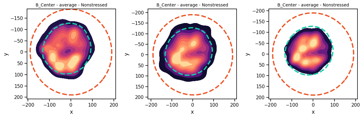
Now, what we are seeing here is all the center positions of the black mouse dependent on if our selected bodyparts were inside the ROI. Respectively, the second plot covers a slightly larger area, as it includes cases where the black mouse stands outside of the ROI and just sticks it’s head in, i.e. it’S Center is outside of the ROI. The third plot covers a slightly smaller area, as absolutely all bodyparts of the black mouse need to be inside of the ROI here.

The roi_functionality works similar for other visualization options, such as the skeleton animation. Here we animate all data for the first 20 seconds (as determined by bin_index and bin_size) during which the black mouse (“B”) is in the top half of the arena, independent of the position of the white mouse (“W”).

from IPython import display

video = deepof.visuals.animate_skeleton(
    my_deepof_project_with_rois,
    experiment_id="20191204_Day2_SI_JB08_Test_54",
    bin_index=0,
    bin_size=20,
    sampling_rate=25,
    dpi=60,
    roi_number=1,
    animals_in_roi="B",
    in_roi_criterion="Center",
)

html = display.HTML(video)
display.display(html)
plt.close()

If we instead want that both mice are inside of the ROI, we can also simply set animals_in_roi using a list.

from IPython import display

video = deepof.visuals.animate_skeleton(
    my_deepof_project_with_rois,
    experiment_id="20191204_Day2_SI_JB08_Test_54",
    bin_index=0,
    bin_size=20,
    sampling_rate=25,
    dpi=60,
    roi_number=1,
    animals_in_roi=["B", "W"],
)

html = display.HTML(video)
display.display(html)
plt.close()

Plotting with ROIs

For most of the other plots we either need supervised or unsupervised annotations, so let’s quickly compute just that

supervised_annotation = my_deepof_project_with_rois.supervised_annotation()

data preprocessing            : 100%|██████████| 4/4 [00:41<00:00, 10.45s/step, step=Loading kinematics]
supervised annotations        : 100%|██████████| 53/53 [01:28<00:00,  1.67s/table, step=post processing]

Now we can apply ROIs to Gant plots, Enrichment plots, and more.

plt.figure(figsize=(12, 8))

deepof.visuals.plot_gantt(
    my_deepof_project_with_rois,
    "20191204_Day2_SI_JB08_Test_54",
    supervised_annotations=supervised_annotation,
    roi_number=1,
    animals_in_roi=["B","W"],
)

plt.show()

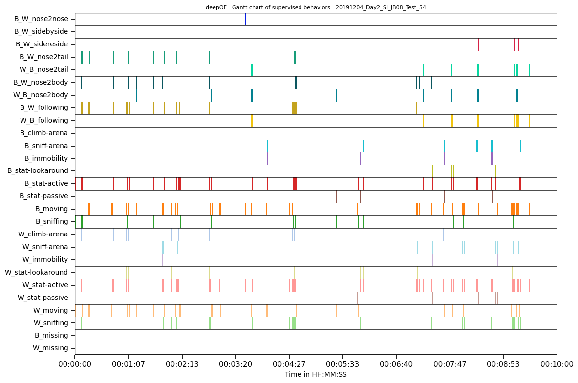
This Gantt-plot is a lot more sparse than it’s pendant in the supervised tutorial, which is expected, as we only include frames during which both mice are in the upper half of the arena.

Some plots like plot_enrichment have an additional roi setting specifically for supervised annotations.

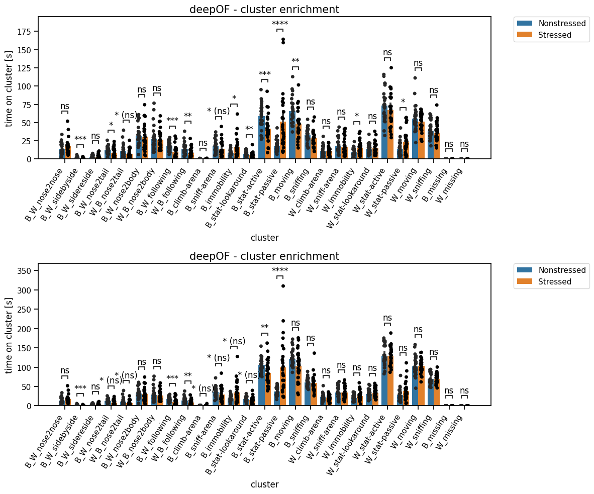
• The roi_mode is always set to “mousewise” as a default. This means that the ROIs behave exactly as in all examples before, occuring behaviors are only included if the animals given in animals_in_roi were inside of the ROI during that time. If no animals_in_roi input is explicietly given, all available animals need to be inside of the ROI.

• If the roi_mode is set to “behaviorwise” instead, the animals_in_roi input is ignored. Now all behaviors are included during which the mice taking part in that behavior were inside of the ROI. This means that for e.g. B_immobility it is only relevant that the black mouse was inside of the ROI during detection. For W_immobility only the white mouse needs to be inside of the ROI and for paired behaviors, such as W_B_following, both mice need to be inside of the ROI.

fig, (ax1, ax2) = plt.subplots(2, 1, figsize=(12, 10))

deepof.visuals.plot_enrichment(
    my_deepof_project_with_rois,
    supervised_annotations=supervised_annotation,
    add_stats="Mann-Whitney",
    plot_speed=False,
    roi_number = 1,
    roi_mode = "mousewise",
    animals_in_roi=["B","W"],
    ax = ax1,
)

deepof.visuals.plot_enrichment(
    my_deepof_project_with_rois,
    supervised_annotations=supervised_annotation,
    add_stats="Mann-Whitney",
    plot_speed=False,
    roi_number = 1,
    roi_mode = "behaviorwise",
    ax = ax2,
)

plt.tight_layout()
plt.show()

Other plot functions, such as plot_transitions, plot_stationary_entropy, plot_embeddings or plot_behavior_trends as well as export_annotated_video also support the roi functionality. Besides applying ROIs on the existing plotting functions, there is also specific ROI-related information that can be visualized.

ROI specific plots

The function “plot_mouse_roi_interaction” allows the user to visualize the distances different mice from different ROIs have. It works analogously to plot_behavior_trends (see Supervised tutorial) by showing the average distance for chosen time bins of given mouse bodyparts to a given ROI. If more than one bodypart is given, the distance to the bodypart closest to the ROI is counted. With the call below we evaluate the distance of the nose of the black mouse to ROI 3 (the inner arena circle) for 20 time bins accross teh signal, compairing the CSDS conditions. Note that the distance is ignored if the mouse bodypart is inside of the ROI.

deepof.visuals.plot_mouse_roi_interaction(
    my_deepof_project_with_rois,
    bodyparts = ["B_Nose"],
    roi_number= 3,
    N_time_bins=20,
    mode="distance",
    exp_condition="CSDS",
)

plt.show()

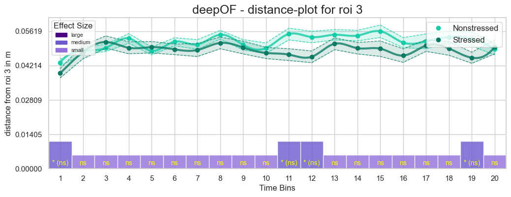
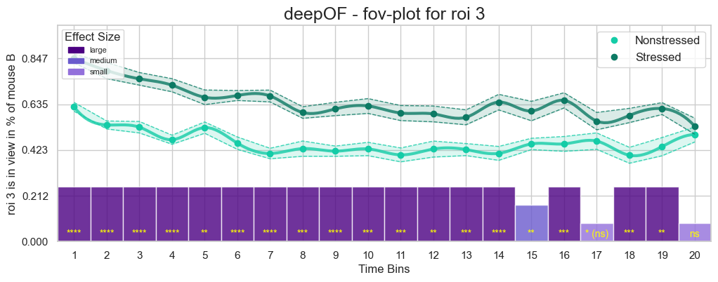
As we can see there is not much of a difference, only the nose of the black mouse might, on average, be slightly closer to the ROI (if the mouse is not inside the ROI). This seems odd at first, as we also know that the stressed mice in general avoid the middle of the arena. But there is an explanation for this. Now, if we switch to the “field of view” (i.e. “fov”) mode and sleect an animal id instead, we can now visualize how long roi 3 was in the field of view of the black mouse for the stressed and non-stressed case.

deepof.visuals.plot_mouse_roi_interaction(
    my_deepof_project_with_rois,
    animal_id = "B",
    roi_number= 3,
    N_time_bins=20,
    mode="fov",
    exp_condition="CSDS",
)

<Axes: title={'center': 'deepOF - fov-plot for roi 3'}, xlabel='Time Bins', ylabel='roi 3 is in view in % of mouse B'>

With this we now clearly see that the stressed mice were looking more often towards ROI 3, i.e. the center of the arena, especially towards the beginning of the experiment. This makes sense, as a stressed mouse might be more anxious about keeping an eye on the dominant mouse. The direction in which the mouse is looking is likely also the reason for the slight difference in nose distances.

Additionally, the plotted data can be returned directly by using the function return_mouse_roi_interaction. It uses mostly the same input options as the plot function and returns two tables per default

binned_effect_sizes_df, binned_group_df = deepof.visuals.return_mouse_roi_interaction(
    my_deepof_project_with_rois,
    animal_id = "B",
    roi_number= 3,
    N_time_bins=20,
    mode="fov",
    exp_condition="CSDS",
)

binned_effect_sizes_df contains all plotted information including effect sizes.

binned_effect_sizes_df

	time_bin	Absolute_Cohens_d	Effect_Size_Category	bin_means_Nonstressed	bin_sem_Nonstressed	bin_means_Stressed	bin_sem_Stressed
0	0	2.147370	3	0.623332	0.020562	0.846828	0.019887
1	1	1.641865	3	0.539462	0.018466	0.791246	0.037320
2	2	1.555294	3	0.529122	0.026582	0.752996	0.029172
3	3	1.863716	3	0.471120	0.021082	0.723351	0.030317
4	4	0.897202	3	0.527192	0.026131	0.667511	0.033834
5	5	1.652882	3	0.455210	0.028639	0.675814	0.023123
6	6	1.995586	3	0.407317	0.024271	0.673574	0.027347
7	7	1.040807	3	0.429874	0.035301	0.597100	0.026862
8	8	1.373401	3	0.418158	0.023645	0.613590	0.030877
9	9	1.180728	3	0.428277	0.030910	0.627180	0.034308
10	10	1.120252	3	0.400932	0.032131	0.594618	0.034868
11	11	0.859580	3	0.427903	0.036961	0.590536	0.036547
12	12	0.919912	3	0.425534	0.027857	0.574910	0.034599
13	13	1.346581	3	0.407891	0.032162	0.645142	0.036020
14	14	0.795597	2	0.451670	0.026151	0.603879	0.045010
15	15	1.127227	3	0.451806	0.034309	0.653350	0.035108
16	16	0.458690	1	0.464717	0.038098	0.557228	0.040140
17	17	1.025630	3	0.399075	0.036809	0.583382	0.033038
18	18	0.968263	3	0.439136	0.042203	0.615334	0.027506
19	19	0.208054	1	0.495226	0.034547	0.533786	0.037289

And binned_group_df contains the group and binning information for all included experiments and experimental conditions.

binned_group_df

	time_bin	bin_length	exp_condition	fov
0	0	730	Nonstressed	0.491108
1	1	730	Nonstressed	0.522222
2	2	730	Nonstressed	0.678977
3	3	730	Nonstressed	0.627907
4	4	730	Nonstressed	0.745554
...	...	...	...	...
1055	15	730	Stressed	0.807114
1056	16	730	Stressed	0.683562
1057	17	730	Stressed	0.567308
1058	18	730	Stressed	0.484225
1059	19	730	Stressed	0.834247

1060 rows × 4 columns

Alternatively, raw data of only field of view or distance information can be directly retrieved for all experimental conditions, ignoring all binning

deepof.visuals.return_mouse_roi_interaction(
    my_deepof_project_with_rois,
    animal_id = "B",
    roi_number= 3,
    N_time_bins=20,
    mode="fov",
    exp_condition="CSDS",
    get_raw_data=True
)

	20191203_Day1_SI_JB08_Test_7	20191203_Day1_SI_JB08_Test_8	20191203_Day1_SI_JB08_Test_13	20191203_Day1_SI_JB08_Test_14	20191203_Day1_SI_JB08_Test_23	20191203_Day1_SI_JB08_Test_24	20191203_Day1_SI_JB08_Test_29	20191203_Day1_SI_JB08_Test_30	20191203_Day1_SI_JB08_Test_39	20191203_Day1_SI_JB08_Test_40	...	20191204_Day2_SI_JB08_Test_24	20191204_Day2_SI_JB08_Test_30	20191204_Day2_SI_JB08_Test_39	20191204_Day2_SI_JB08_Test_40	20191204_Day2_SI_JB08_Test_45	20191204_Day2_SI_JB08_Test_46	20191204_Day2_SI_JB08_Test_55	20191204_Day2_SI_JB08_Test_56	20191204_Day2_SI_JB08_Test_61	20191204_Day2_SI_JB08_Test_62
0	1.0	0.0	1.0	1.0	1.0	1.0	1.0	1.0	0.0	0.0	...	1.0	NaN	1.0	1.0	1.0	1.0	0.0	1.0	1.0	1.0
1	1.0	0.0	1.0	1.0	1.0	1.0	1.0	1.0	0.0	0.0	...	1.0	NaN	1.0	1.0	1.0	1.0	0.0	1.0	1.0	1.0
2	1.0	0.0	1.0	1.0	1.0	1.0	1.0	1.0	0.0	0.0	...	1.0	NaN	1.0	1.0	1.0	1.0	0.0	1.0	1.0	1.0
3	1.0	0.0	1.0	1.0	1.0	1.0	1.0	1.0	0.0	0.0	...	1.0	NaN	1.0	1.0	1.0	1.0	0.0	1.0	1.0	1.0
4	1.0	0.0	1.0	1.0	1.0	1.0	1.0	1.0	0.0	0.0	...	1.0	NaN	1.0	1.0	1.0	1.0	0.0	1.0	1.0	1.0
...	...	...	...	...	...	...	...	...	...	...	...	...	...	...	...	...	...	...	...	...	...
14996	1.0	0.0	1.0	NaN	0.0	0.0	1.0	0.0	0.0	1.0	...	0.0	0.0	0.0	1.0	0.0	1.0	1.0	1.0	0.0	0.0
14997	1.0	0.0	NaN	NaN	NaN	NaN	1.0	0.0	NaN	1.0	...	0.0	NaN	0.0	NaN	0.0	1.0	1.0	1.0	0.0	0.0
14998	NaN	NaN	NaN	NaN	NaN	NaN	1.0	0.0	NaN	NaN	...	NaN	NaN	0.0	NaN	0.0	NaN	1.0	NaN	0.0	NaN
14999	NaN	NaN	NaN	NaN	NaN	NaN	1.0	0.0	NaN	NaN	...	NaN	NaN	0.0	NaN	NaN	NaN	NaN	NaN	NaN	NaN
15000	NaN	NaN	NaN	NaN	NaN	NaN	NaN	NaN	NaN	NaN	...	NaN	NaN	NaN	NaN	NaN	NaN	NaN	NaN	NaN	NaN

15001 rows × 53 columns

Analogously ROIs can also be applied to other data sources.

Extract data directly using ROIs

Plotting all of this may look nice, but maybe you want to create your own, even nicer plot. For this we have various ways to extract data directly after ROI application

Extracting coordinates works exactly as described in the preprocessing tutorial. It only requires the addition of the roi_number you want to use and the animals that should be inside of that ROI. Aditonally you can also set a in_roi_criterion just as you can for teh plots. All frames during which these conditions were not fulfilled will be set to NaN.

coords = my_deepof_project_with_rois.get_coords(roi_number=1, animals_in_roi=["B","W"], in_roi_criterion="Center")
coords.filter_id("B")['20191204_Day2_SI_JB08_Test_54']

	B_Center		B_Left_bhip		B_Left_ear		B_Left_fhip		B_Nose		...	B_Right_ear		B_Right_fhip		B_Spine_1		B_Spine_2		B_Tail_base
	x	y	x	y	x	y	x	y	x	y	...	x	y	x	y	x	y	x	y	x	y
00:00:00	178.695067	150.903525	178.133481	164.579831	160.236194	129.369839	162.932410	149.543005	166.288734	115.459213	...	175.473650	127.391220	181.920601	137.218331	170.050867	140.762637	190.880247	157.459358	204.986693	161.780679
00:00:00.040002666	178.695067	150.903525	178.133481	164.579831	160.236194	129.369839	162.932410	149.543005	166.288734	115.459213	...	175.473650	127.391220	181.920601	137.218331	170.050867	140.762637	190.880247	157.459358	204.986693	161.780679
00:00:00.080005333	178.695067	150.903525	178.133481	164.579831	160.236194	129.369839	162.932410	149.543005	166.288734	115.459213	...	175.473650	127.391220	181.920601	137.218331	170.050867	140.762637	190.880247	157.459358	204.986693	161.780679
00:00:00.120008	177.009679	149.650528	175.106624	163.666017	163.807836	124.262824	161.761900	147.278549	174.192032	112.040097	...	180.079795	125.958622	184.009635	136.824217	171.210362	138.769813	188.593896	157.714930	203.863200	162.280499
00:00:00.160010667	177.767518	147.833830	173.779126	162.437004	167.520924	121.969513	163.445137	144.056996	179.274246	108.299092	...	183.599288	123.947488	186.337662	135.377970	173.565589	136.397291	187.809489	157.195280	202.295015	162.775274
...	...	...	...	...	...	...	...	...	...	...	...	...	...	...	...	...	...	...	...	...	...
00:09:59.799986665	NaN	NaN	NaN	NaN	NaN	NaN	NaN	NaN	NaN	NaN	...	NaN	NaN	NaN	NaN	NaN	NaN	NaN	NaN	NaN	NaN
00:09:59.839989332	NaN	NaN	NaN	NaN	NaN	NaN	NaN	NaN	NaN	NaN	...	NaN	NaN	NaN	NaN	NaN	NaN	NaN	NaN	NaN	NaN
00:09:59.879991999	NaN	NaN	NaN	NaN	NaN	NaN	NaN	NaN	NaN	NaN	...	NaN	NaN	NaN	NaN	NaN	NaN	NaN	NaN	NaN	NaN
00:09:59.919994666	NaN	NaN	NaN	NaN	NaN	NaN	NaN	NaN	NaN	NaN	...	NaN	NaN	NaN	NaN	NaN	NaN	NaN	NaN	NaN	NaN
00:09:59.959997333	NaN	NaN	NaN	NaN	NaN	NaN	NaN	NaN	NaN	NaN	...	NaN	NaN	NaN	NaN	NaN	NaN	NaN	NaN	NaN	NaN

14999 rows × 22 columns

For merging tables, one should take care to enter the correct arguments in both data retrival function calls. Otherwise missmatches can happen, as in this example, in which different roi numbers were used for the standard coords and distance tables.

my_deepof_project_with_rois.get_coords(roi_number=1, animals_in_roi=["B","W"]).merge(my_deepof_project_with_rois.get_areas(roi_number=2, animals_in_roi=["B","W"]))['20191204_Day2_SI_JB08_Test_54']

	(B_Center, x)	(B_Center, y)	(B_Left_bhip, x)	(B_Left_bhip, y)	(B_Left_ear, x)	(B_Left_ear, y)	(B_Left_fhip, x)	(B_Left_fhip, y)	(B_Nose, x)	(B_Nose, y)	...	(W_Tail_base, x)	(W_Tail_base, y)	B_head_area	B_torso_area	B_back_area	B_full_area	W_head_area	W_torso_area	W_back_area	W_full_area
00:00:00	178.695067	150.903525	178.133481	164.579831	160.236194	129.369839	162.932410	149.543005	166.288734	115.459213	...	284.276209	81.953327	NaN	NaN	NaN	NaN	NaN	NaN	NaN	NaN
00:00:00.040002666	178.695067	150.903525	178.133481	164.579831	160.236194	129.369839	162.932410	149.543005	166.288734	115.459213	...	284.276209	81.953327	NaN	NaN	NaN	NaN	NaN	NaN	NaN	NaN
00:00:00.080005333	178.695067	150.903525	178.133481	164.579831	160.236194	129.369839	162.932410	149.543005	166.288734	115.459213	...	284.276209	81.953327	NaN	NaN	NaN	NaN	NaN	NaN	NaN	NaN
00:00:00.120008	177.009679	149.650528	175.106624	163.666017	163.807836	124.262824	161.761900	147.278549	174.192032	112.040097	...	293.070473	82.577959	NaN	NaN	NaN	NaN	NaN	NaN	NaN	NaN
00:00:00.160010667	177.767518	147.833830	173.779126	162.437004	167.520924	121.969513	163.445137	144.056996	179.274246	108.299092	...	299.036433	86.246318	NaN	NaN	NaN	NaN	NaN	NaN	NaN	NaN
...	...	...	...	...	...	...	...	...	...	...	...	...	...	...	...	...	...	...	...	...	...
00:09:59.799986665	NaN	NaN	NaN	NaN	NaN	NaN	NaN	NaN	NaN	NaN	...	NaN	NaN	239.351756	336.178223	369.570164	1236.107578	338.985792	306.291532	398.589194	1296.123237
00:09:59.839989332	NaN	NaN	NaN	NaN	NaN	NaN	NaN	NaN	NaN	NaN	...	NaN	NaN	225.022660	337.583006	356.664988	1202.726262	339.620050	307.614990	401.612088	1299.472646
00:09:59.879991999	NaN	NaN	NaN	NaN	NaN	NaN	NaN	NaN	NaN	NaN	...	NaN	NaN	254.932272	347.361879	366.539329	1240.353140	339.318562	307.496487	402.713953	1300.378284
00:09:59.919994666	NaN	NaN	NaN	NaN	NaN	NaN	NaN	NaN	NaN	NaN	...	NaN	NaN	254.932272	347.361879	366.539329	1240.353140	339.318562	307.496487	402.713953	1300.378284
00:09:59.959997333	NaN	NaN	NaN	NaN	NaN	NaN	NaN	NaN	NaN	NaN	...	NaN	NaN	254.932272	347.361879	366.539329	1240.353140	339.318562	307.496487	402.713953	1300.378284

14999 rows × 52 columns

Similarily, we can also count events using ROIs

deepof.visuals.count_all_events(
    my_deepof_project_with_rois,
    supervised_annotations=supervised_annotation,
    bin_size=60,
    bin_index=0,
    counting_mode = "Events",
    roi_number=1,
    animals_in_roi="B",
)

	B_W_nose2nose	B_W_sidebyside	B_W_sidereside	B_W_nose2tail	W_B_nose2tail	B_W_nose2body	W_B_nose2body	B_W_following	W_B_following	B_climb-arena	...	W_moving	W_sniffing	B_missing	W_missing	B_distance	B_cum-distance	B_speed	W_distance	W_cum-distance	W_speed
20191203_Day1_SI_JB08_Test_5	1	0	0	0	0	0	0	0	1	0	...	25	74	0	0	NaN	NaN	NaN	NaN	NaN	NaN
20191203_Day1_SI_JB08_Test_6	3	0	1	0	2	3	4	0	3	0	...	14	31	0	0	NaN	NaN	NaN	NaN	NaN	NaN
20191203_Day1_SI_JB08_Test_7	1	0	1	6	1	3	2	5	3	0	...	11	26	0	0	NaN	NaN	NaN	NaN	NaN	NaN
20191203_Day1_SI_JB08_Test_8	5	4	1	8	1	10	2	9	1	0	...	14	34	0	0	NaN	NaN	NaN	NaN	NaN	NaN
20191203_Day1_SI_JB08_Test_13	2	0	1	0	1	4	2	3	0	0	...	16	30	0	0	NaN	NaN	NaN	NaN	NaN	NaN
20191203_Day1_SI_JB08_Test_14	4	0	0	3	0	9	1	3	1	0	...	22	48	0	0	NaN	NaN	NaN	NaN	NaN	NaN
20191203_Day1_SI_JB08_Test_15	7	0	0	0	2	6	6	0	1	0	...	23	53	0	0	NaN	NaN	NaN	NaN	NaN	NaN
20191203_Day1_SI_JB08_Test_16	1	0	0	0	2	1	3	0	1	0	...	25	59	0	0	NaN	NaN	NaN	NaN	NaN	NaN
20191203_Day1_SI_JB08_Test_22	1	0	0	0	0	0	1	0	0	0	...	28	59	0	0	NaN	NaN	NaN	NaN	NaN	NaN
20191203_Day1_SI_JB08_Test_23	0	0	0	7	0	9	0	7	0	0	...	8	21	0	0	NaN	NaN	NaN	NaN	NaN	NaN
20191203_Day1_SI_JB08_Test_24	1	0	0	6	0	8	1	6	0	0	...	8	23	0	0	NaN	NaN	NaN	NaN	NaN	NaN
20191203_Day1_SI_JB08_Test_29	4	0	1	8	6	12	10	7	7	0	...	15	47	0	0	NaN	NaN	NaN	NaN	NaN	NaN
20191203_Day1_SI_JB08_Test_30	2	0	1	16	0	11	3	13	3	0	...	12	32	0	1	NaN	NaN	NaN	NaN	NaN	NaN
20191203_Day1_SI_JB08_Test_31	3	0	0	0	1	2	1	0	1	0	...	7	16	0	0	NaN	NaN	NaN	NaN	NaN	NaN
20191203_Day1_SI_JB08_Test_32	0	0	0	0	0	0	0	0	0	0	...	0	0	0	0	0.0	0.0	0.0	0.0	0.0	0.0
20191203_Day1_SI_JB08_Test_37	1	0	0	0	0	0	0	0	1	0	...	22	53	0	0	NaN	NaN	NaN	NaN	NaN	NaN
20191203_Day1_SI_JB08_Test_38	3	0	0	0	1	1	2	0	4	0	...	19	51	0	0	NaN	NaN	NaN	NaN	NaN	NaN
20191203_Day1_SI_JB08_Test_39	1	0	4	6	4	6	3	9	6	0	...	12	49	0	1	NaN	NaN	NaN	NaN	NaN	NaN
20191203_Day1_SI_JB08_Test_40	3	0	3	4	5	7	5	7	5	0	...	27	66	0	0	NaN	NaN	NaN	NaN	NaN	NaN
20191203_Day1_SI_JB08_Test_45	5	2	0	14	1	9	1	14	1	0	...	11	31	0	0	NaN	NaN	NaN	NaN	NaN	NaN
20191203_Day1_SI_JB08_Test_46	1	0	0	6	0	7	1	13	1	0	...	19	42	0	0	NaN	NaN	NaN	NaN	NaN	NaN
20191203_Day1_SI_JB08_Test_47	0	0	0	0	0	0	0	0	0	0	...	7	12	0	0	NaN	NaN	NaN	NaN	NaN	NaN
20191203_Day1_SI_JB08_Test_53	0	0	0	0	0	0	0	0	0	0	...	25	47	0	0	NaN	NaN	NaN	NaN	NaN	NaN
20191203_Day1_SI_JB08_Test_54	4	1	1	7	0	5	1	7	1	0	...	19	43	0	0	NaN	NaN	NaN	NaN	NaN	NaN
20191203_Day1_SI_JB08_Test_55	0	0	0	8	0	6	0	9	0	0	...	13	31	0	0	NaN	NaN	NaN	NaN	NaN	NaN
20191203_Day1_SI_JB08_Test_56	3	0	2	7	2	8	3	3	1	0	...	16	51	0	0	NaN	NaN	NaN	NaN	NaN	NaN
20191204_Day2_SI_JB08_Test_6	0	0	0	4	0	4	0	3	0	0	...	15	45	0	0	NaN	NaN	NaN	NaN	NaN	NaN
20191204_Day2_SI_JB08_Test_7	0	0	0	0	0	0	0	0	2	0	...	12	22	0	0	NaN	NaN	NaN	NaN	NaN	NaN
20191204_Day2_SI_JB08_Test_8	4	0	2	0	3	5	1	0	5	0	...	12	48	0	0	NaN	NaN	NaN	NaN	NaN	NaN
20191204_Day2_SI_JB08_Test_13	3	0	1	0	1	2	3	0	4	0	...	15	37	0	0	NaN	NaN	NaN	NaN	NaN	NaN
20191204_Day2_SI_JB08_Test_14	1	0	0	0	0	1	1	0	1	0	...	19	47	0	1	NaN	NaN	NaN	NaN	NaN	NaN
20191204_Day2_SI_JB08_Test_15	3	0	0	5	0	9	1	13	3	0	...	14	32	0	0	NaN	NaN	NaN	NaN	NaN	NaN
20191204_Day2_SI_JB08_Test_16	4	0	3	5	2	11	6	6	4	0	...	11	28	0	0	NaN	NaN	NaN	NaN	NaN	NaN
20191204_Day2_SI_JB08_Test_21	2	1	2	8	3	10	4	11	3	0	...	11	32	0	0	NaN	NaN	NaN	NaN	NaN	NaN
20191204_Day2_SI_JB08_Test_22	2	3	1	12	0	14	0	13	0	0	...	17	45	0	0	NaN	NaN	NaN	NaN	NaN	NaN
20191204_Day2_SI_JB08_Test_23	1	0	0	0	0	1	2	0	2	0	...	8	12	0	0	NaN	NaN	NaN	NaN	NaN	NaN
20191204_Day2_SI_JB08_Test_24	0	0	0	0	0	0	0	0	2	0	...	26	48	0	0	NaN	NaN	NaN	NaN	NaN	NaN
20191204_Day2_SI_JB08_Test_30	7	0	0	0	0	3	8	0	0	0	...	38	89	0	0	NaN	NaN	NaN	NaN	NaN	NaN
20191204_Day2_SI_JB08_Test_37	1	0	2	7	3	7	4	9	4	0	...	22	60	0	0	NaN	NaN	NaN	NaN	NaN	NaN
20191204_Day2_SI_JB08_Test_38	0	1	2	6	1	9	4	6	3	0	...	15	32	0	0	NaN	NaN	NaN	NaN	NaN	NaN
20191204_Day2_SI_JB08_Test_39	2	1	0	4	1	11	3	6	1	0	...	13	29	0	0	NaN	NaN	NaN	NaN	NaN	NaN
20191204_Day2_SI_JB08_Test_40	0	0	1	0	0	0	0	0	0	0	...	3	6	0	0	NaN	NaN	NaN	NaN	NaN	NaN
20191204_Day2_SI_JB08_Test_45	1	0	0	0	0	0	1	0	0	0	...	19	30	0	0	NaN	NaN	NaN	NaN	NaN	NaN
20191204_Day2_SI_JB08_Test_46	0	0	0	0	0	1	0	0	0	0	...	13	26	0	0	NaN	NaN	NaN	NaN	NaN	NaN
20191204_Day2_SI_JB08_Test_47	2	0	1	1	0	3	2	2	1	0	...	6	25	0	0	NaN	NaN	NaN	NaN	NaN	NaN
20191204_Day2_SI_JB08_Test_53	2	1	2	4	1	8	3	5	2	0	...	27	68	0	0	NaN	NaN	NaN	NaN	NaN	NaN
20191204_Day2_SI_JB08_Test_54	4	0	0	5	0	8	2	5	0	0	...	14	42	0	0	NaN	NaN	NaN	NaN	NaN	NaN
20191204_Day2_SI_JB08_Test_55	0	0	0	0	0	0	0	0	9	0	...	11	24	0	0	NaN	NaN	NaN	NaN	NaN	NaN
20191204_Day2_SI_JB08_Test_56	0	0	0	0	0	0	0	0	0	0	...	19	50	0	0	NaN	NaN	NaN	NaN	NaN	NaN
20191204_Day2_SI_JB08_Test_61	5	0	1	1	1	5	8	0	1	0	...	27	65	0	0	NaN	NaN	NaN	NaN	NaN	NaN
20191204_Day2_SI_JB08_Test_62	4	0	3	1	1	4	4	1	0	0	...	28	67	0	0	NaN	NaN	NaN	NaN	NaN	NaN
20191204_Day2_SI_JB08_Test_63	1	1	0	7	0	9	3	8	3	0	...	15	51	0	0	NaN	NaN	NaN	NaN	NaN	NaN
20191204_Day2_SI_JB08_Test_64	1	1	0	4	1	4	1	5	1	0	...	17	43	0	0	NaN	NaN	NaN	NaN	NaN	NaN

53 rows × 33 columns

Wrapping up

Thank you for making it until the end. In general ROIs can be applied to most functions for which it makes sense. In future updates we are going to implement some options that will enable automatic ROI creations based on requirements such as “the inner 70% of the area”. So stay tuned.