Formatting your data: feature extraction from motion tracking output

What we’ll cover:

• Create and run a project.

• Load a previously generated project.

• Interact with your project: generate coordinates, distances, angles, and areas.

• Exploratory visualizations: heatmaps and processed animations.

# # If using Google colab, uncomment and run this cell and the one below to set up the environment
# # Note: because of how colab handles the installation of local packages, this cell will kill your runtime.
# # This is not an error! Just continue with the cells below.
# import os
# !git clone -q https://github.com/mlfpm/deepof.git
# !pip install -q -e deepof --progress-bar off
# os.chdir("deepof")
# !curl --output tutorial_files.zip https://datashare.mpcdf.mpg.de/s/TbSrod2fm5jbHfL/download
# !unzip tutorial_files.zip

# import os
# os.chdir("deepof")
# import os, warnings
# warnings.filterwarnings('ignore')

Let’s start by importing some packages. We’ll use python’s os library to handle paths, pickle to load saved objects, pandas to load data frames, and the data entry API within DeepOF, located in deepof.data

import os
import pickle
import deepof.data

We’ll also need some plotting gear:

import deepof.visuals
import matplotlib.pyplot as plt
import seaborn as sns
import pandas as pd

Creating and running a project

With that out of the way, the first thing to do when starting a DeepOF project is to load your videos and DeepLabCut tracking files into a deepof.data.Project object.

Like depicted in the cell below, the three crucial parameters to input are the project, video and tab paths.

• project_path specifies where the project folder containing all processing and output files will be created.

• video_path points towards where your DLC or SLEAP labelled videos are stored.

• similarly, table_path should point to the directory containing all tracking files (see section on supported input files below).

• last but not least, you can give your project a name (optional; deepof_project by default).

The dataset used in this tutorial is a subset of the social interaction (SI) dataset used in DeepOF’s original paper. It contains six 10-minute-long videos with two animals (a C57Bl6 and a CD1) tracked in a round arena, tracked with DeepLabCut. Three of the C57Bl6 mice have been exposed to chronic social defeat stress (CSDS).

my_deepof_project_raw = deepof.data.Project(
    project_path=os.path.join("tutorial_files"),
    video_path=os.path.join("tutorial_files/Videos/"),
    table_path=os.path.join("tutorial_files/Tables/"),
    project_name="deepof_tutorial_project",
    arena="circular-autodetect",
    animal_ids=["B", "W"],
    table_format="h5",
    video_format=".mp4",
    exclude_bodyparts=["Tail_1", "Tail_2", "Tail_tip"],
    video_scale="380 mm",
    iterative_imputation="partial",  # "full",
    smooth_alpha=1,
    exp_conditions=None,
    # number_of_rois=3, # another optional input argument that allows you to define up to 20 different regions of interest during project creation
)

Info! Set arena dimension to 380.0 mm!

The sampling rate of some of your videos differ. The maximum difference is 20191204_Day2_SI_JB08_Test_54: 24.99 fps and 20191204_Day2_SI_JB08_Test_63: 24.994 fps! Proceed with cauthion

As you may see, there are some extra (optional) parameters in the call above. These specify some details on how the videos and tracks will be processed. Some include:

• arena: some functions within DeepOF (as you will see in the next tutorial on supervised annotations) require the program to detect the arena. The following section explains how to handle this step in more detail.

• animal_ids: in case more than one animal is present in the dataset, the IDs assigned to each during tracking need to be specified as a list. For SLEAP projects, this will be detected automatically, but can be overriten.

• exclude_body_parts: while DeepOF originally relies on 14 body part tracking models, body parts along the tail are no longer used. This step could be bypassed using smaller models following an 11-body-part scheme, such as the one presented in the landing page of the documentation. Custom labelling schemes are also supported (see tutorials).

• video_scale: diameter of the arena (in mm) if circular. In the case of polygonal arenas, the length (in mm) of the first edge as specified in the GUI (see next section) should be provided.

• smooth_alpha: smoothing intensity. The higher the value, the more smoothing is applied.

• exp_conditions: dictionary with a video IDs as keys, and data frames with all experimental conditions as values. DeepOF will use this information to enable all sorts of comparisons between conditions, as we will see in the following tutorials. We’ll leave it blank for now and update it afterwards.

For more details, feel free to visit the full API reference.

Let’s then create our first project, by running the .create() method in our newly created object:

my_deepof_project = my_deepof_project_raw.create(force=True)

Setting up project directories...

Preprocessing tables          : 100%|██████████| 6/6 [00:03<00:00,  1.95it/s, file=20191204_D..., step=Saving data]
Detecting arenas              : 100%|██████████| 6/6 [01:30<00:00, 15.02s/arena]
Rescaling tables              : 100%|██████████| 6/6 [00:00<00:00, 561.74table/s]
Computing distances           : 100%|██████████| 6/6 [00:00<00:00,  6.37table/s]
Computing angles              : 100%|██████████| 6/6 [00:00<00:00, 42.10table/s]
Computing areas               : 100%|██████████| 6/6 [00:00<00:00,  6.68table/s]

Done!

NOTE: the force parameter allows DeepOF to override an existing project in the same directory. Use with caution!

NOTE 2: the cell above can take a significant amount of time to run in Google colab. Feel free to skip and continue with the loaded results below.

As you will see, this organizes all required file into a folder in the specified path. Moreover, some processing steps are computed on the go, such as distances, angles and areas. This makes it easier for DeepOF to load all required features later on, without the need to compute them every time.

Arena detection

As mentioned above, one of the key aspects of project creation involves setting up the arena detection mechanism, which will be used in downstream tasks, such as climbing detection and overall video scaling.

You can contrAlong these lines, the package provides tools for detecting elliptical arenas specifically (as seen in this tutorial), and general polygonal shapes (such as squares, rectangles, Y-mazes, etc).

In principle, DeepOF can detect your arenas automatically by relying in SAM (Segment Anything Model), a state-of-the-art image segmentation deep learning model. By selecting arena='circular-autodetect', or arena='polygonal-autodetect', users can benefit from this approach. A folder named Arena_detection will be created in your project directory, which contains samples of the detected arenas for all videos, so you can visually inspect if DeepOF did a good job.

Moreover, manual annotation can be selected using arena='circular-manual', and arena='polygonal-manual'. In this case, you will see a window per video appear, allowing you to manually mark where the arena is with just a few clicks. All results will be stored for further processing.

Here, clicking anywhere in the video will make an orange marker appear. In the case of polygonal arenas, at least a marker per corner should be used. When dealing with circular (or elliptical) arenas, DeepOF will fit an ellipse to the marked points after a minimum of 5 clicks. The ellipse can always be refined by adding more markers. Once finished with a video, press q to save and move to the next one. If you made a mistake and would like to correct it, press d to delete the last added marker. Moreover, after you tagged at least one video, you’ll see the p option appear, which will copy the last marked arena to all remaining videos in the dataset.

NOTE: If you select arena='polygonal-autodetect', you will still be prompted with the GUI to select the arena just once, so SAM roughly knows how the segmentation it should return looks like. Detection in all remaining videos will be automatic. This is not the case for arena='circular-autodetect', as we already know we’re looking for a circle.

One last thing is that, in polygonal arenas, the first edge you input will be used to scale the coordinates to the proper distances (pixels to millimeters). Make sure you always mark the same edge first, and that it coincides with the length passed to the “video_scale” parameter when creating the project. In saved images of automatically detected polygons, you’ll see orange circles marking two arena corners. These should match the first edge you selected when prompting SAM, ensuring data is properly scaled.

If after all this work you make a mistake while labelling, or see that automatic detection failed in some cases, don’t worry! You can always edit manually annotated arenas (or rerun automatic annotation) for specific videos using the .edit_arenas() method. Just pass a list with the IDs of the videos you would like to relabel, and the GUI will pop up once again. The same methods described above can be passed to the arena_type parameter.

NOTE: If you don’t pass any video IDs, all videos will be selected by default.

my_deepof_project.edit_arenas(
    video_keys=['20191204_Day2_SI_JB08_Test_54', '20191204_Day2_SI_JB08_Test_62'],
    arena_type="circular-autodetect",
)

Editing 2 arenas

Detecting arenas              : 100%|██████████| 2/2 [00:02<00:00,  1.17s/arena]

Done!

Supported input tracking files:

DeepOF currently supports input from both DeepLabCut and SLEAP. While DeepOF will try to detect automatically which file type you’re trying to use, this can be forced with the table_format parameter in the deepof.data.Project() call depicted in the previous section.

For DeepLabCut, we support:

• Single and multi-animal project CSV files (indicated simply with table_format='csv'.

• Single and multi-animal project h5 files (indicated simply with table_format='h5'.

For SLEAP, you can use:

• SLP files (indicated as with table_format='slp'.

• Raw .npy files (indicated with table_format='npy'.

• h5 files (indicated with table_format=analysis.h5.

Downstream processing should be identical regardless of the files selected, as DeepOF internally brings all these inputs into an equivalent representation. Let’s continue!

Loading a previously generated project

Once you ran your project at least once, it can be loaded without much effort from the path you specified in the first place (plus the project name -deepof_project, if you didn’t specify otherwise-).

# Load a previously saved project
my_deepof_project = deepof.data.load_project("./tutorial_files/deepof_tutorial_project/")

Extend a previously generated project

If you’d like to add data (videos and tracks) to a previously processed project, you can create a new project with the extend method as an alternative to create. For this, you simply define a new project at first that contains the paths to the videos and tables you want to add.

my_new_deepof_project_raw = deepof.data.Project(
    project_path=os.path.join("tutorial_files"),
    video_path=os.path.join("tutorial_files/Videos/"), # This could be new table and video paths to new tables and videos
    table_path=os.path.join("tutorial_files/Tables/"), # For this tutorial we only use the same paths to avoid inflating the tutorial materials even more
    project_name="deepof_tutorial_project",
    arena="circular-autodetect",
    animal_ids=["B", "W"],
    table_format="h5",
    video_format=".mp4",
    exclude_bodyparts=["Tail_1", "Tail_2", "Tail_tip"],
    video_scale="380 mm",
    iterative_imputation="partial",  # "full",
    smooth_alpha=1,
    exp_conditions=None,
)

Info! Set arena dimension to 380.0 mm!

The sampling rate of some of your videos differ. The maximum difference is 20191204_Day2_SI_JB08_Test_54: 24.99 fps and 20191204_Day2_SI_JB08_Test_63: 24.994 fps! Proceed with cauthion

Now you can call the extend method on this new raw project with a path to your old project. What now happens is that tables and videos of your old project get copied over and teh project get’S recreated with teh settings you specified in your new raw project “my_new_deepof_project_raw”.

NOTE: Your old files will not be deleted.

# Extend a previously saved project
my_deepof_project=my_new_deepof_project_raw.extend(
    "./tutorial_files/deepof_tutorial_project/",)

Loading previous project...
Processing data from 0 experiments...

Interacting with your project: generating coordinates, distances, angles, and areas.

That’s it for basic project creation. We now have a DeepOF project up and running! Before ending the tutorial, however, let’s explore the object that the commands above produced.

For starters, if we print it, we see it’s a DeepOF analysis of 6 videos. Furthermore, the object belongs to a custom class within DeepOF, called Coordinates. This class allows the package to store all sorts of relevant information required for further processing, as we’ll see below:

print(my_deepof_project)
print(type(my_deepof_project))

deepof analysis of 6 videos
<class 'deepof.data.Coordinates'>

As described before, the .create() method runs most of the heavy preprocessing already, which allows us to extract features including coordinates, distances, angles, and areas. Let’s see how that works!

With the .get_coords() method, for example, we can obtain the processed (smooth and imputed) tracks for all videos in a dictionary. The returned objects are called table dictionaries (TableDict is the name of the class). They follow a dictionary-like structure, where each value is a data frame. They also provide a plethora of extra methods, some of which we’ll cover in these tutorials. Let’s retrieve these for one of the animals:

my_deepof_project.get_coords(polar=False, center="Center", align="Spine_1")['20191204_Day2_SI_JB08_Test_54']

	B_Spine_1		B_Center		B_Left_bhip		B_Left_ear		B_Left_fhip		...	W_Right_bhip		W_Right_ear		W_Right_fhip		W_Spine_2		W_Tail_base
	x	y	x	y	x	y	x	y	x	y	...	x	y	x	y	x	y	x	y	x	y
00:00:00	0.0	13.268574	0.0	0.0	9.259892	-10.001167	0.078306	28.241925	11.066130	11.213022	...	-12.546447	-11.192675	-10.035840	42.969504	-11.524248	10.333786	0.640064	-17.075071	1.424787	-33.582449
00:00:00.040002666	0.0	13.268574	0.0	0.0	9.259892	-10.001167	0.078306	28.241925	11.066130	11.213022	...	-12.546447	-11.192675	-10.035840	42.969504	-11.524248	10.333786	0.640064	-17.075071	1.424787	-33.582449
00:00:00.080005333	0.0	13.268574	0.0	0.0	9.259892	-10.001167	0.078306	28.241925	11.066130	11.213022	...	-12.546447	-11.192675	-10.035840	42.969504	-11.524248	10.333786	0.640064	-17.075071	1.424787	-33.582449
00:00:00.120008	0.0	12.277365	0.0	0.0	8.236504	-11.424544	-0.289594	28.492124	12.287772	9.225711	...	-11.673510	-13.020497	-9.650663	42.167797	-11.756202	10.658315	1.056564	-17.883001	2.271495	-34.243691
00:00:00.160010667	0.0	12.132295	0.0	0.0	8.742645	-12.279418	0.695124	27.693203	12.089622	8.448482	...	-11.318444	-14.658820	-16.104475	39.924644	-12.021719	9.135641	1.577374	-18.110795	1.847037	-35.836905
...	...	...	...	...	...	...	...	...	...	...	...	...	...	...	...	...	...	...	...	...	...
00:09:59.799986665	0.0	14.024704	0.0	0.0	12.879713	-9.621307	8.597730	28.564627	11.948957	9.096319	...	-16.793977	-5.535776	-13.959892	25.095340	-9.851373	8.488452	-5.071659	-12.336885	-14.884535	-21.557477
00:09:59.839989332	0.0	12.157960	0.0	0.0	12.732978	-10.873408	5.842532	31.657569	11.954985	7.335036	...	-16.886787	-5.682319	-13.971618	25.020048	-9.890848	8.412287	-5.018521	-12.489440	-14.828223	-21.698982
00:09:59.879991999	0.0	15.680413	0.0	0.0	10.365449	-9.330840	6.149816	34.081072	11.982110	9.832851	...	-16.871836	-5.689903	-14.007790	24.969325	-9.874384	8.383054	-4.985731	-12.507850	-14.789899	-21.748366
00:09:59.919994666	0.0	15.680413	0.0	0.0	10.365449	-9.330840	6.149816	34.081072	11.982110	9.832851	...	-16.871836	-5.689903	-14.007790	24.969325	-9.874384	8.383054	-4.985731	-12.507850	-14.789899	-21.748366
00:09:59.959997333	0.0	15.680413	0.0	0.0	10.365449	-9.330840	6.149816	34.081072	11.982110	9.832851	...	-16.871836	-5.689903	-14.007790	24.969325	-9.874384	8.383054	-4.985731	-12.507850	-14.789899	-21.748366

14999 rows × 44 columns

Note that there are a few parameters you can pass to the .get_coords() method. If “polar” is set to True, polar coordinates will be used, instead of Cartesian. Both “center” and “align” control how translational and rotational variance are removed from the data: the former will use the specified body part as [0, 0] (or the center of the arena, if set to “arena”). The latter will rotate the mice on each time point, to align the line connecting the body parts specified in the “center” and “align” parameters with the y-axis.

Furthermore, not only processed coordinates can be retrieved, but also distances, angles, and areas with the .get_distances(), .get_angles(), and .get_areas(), respectively.

my_deepof_project.get_distances()['20191204_Day2_SI_JB08_Test_54']

	(W_Right_ear, W_Spine_1)	(B_Center, B_Spine_2)	(B_Nose, B_Right_ear)	(B_Left_ear, B_Spine_1)	(W_Nose, W_Right_ear)	(W_Left_bhip, W_Spine_2)	(B_Left_ear, B_Nose)	(W_Left_ear, W_Spine_1)	(B_Center, B_Right_fhip)	(B_Tail_base, W_Tail_base)	...	(B_Tail_base, W_Nose)	(B_Nose, W_Tail_base)	(W_Center, W_Left_fhip)	(W_Spine_2, W_Tail_base)	(W_Left_ear, W_Nose)	(B_Right_ear, B_Spine_1)	(W_Right_bhip, W_Spine_2)	(W_Center, W_Right_fhip)	(W_Center, W_Spine_2)	(B_Nose, W_Nose)
00:00:00	25.216999	13.778064	14.993799	14.973556	24.686034	14.389087	15.105907	27.455541	14.000475	112.035495	...	164.593455	122.131897	20.036237	16.526019	22.127720	14.367914	14.439068	15.478871	17.087063	201.683857
00:00:00.040002666	25.216999	13.778064	14.993799	14.973556	24.686034	14.389087	15.105907	27.455541	14.000475	112.035495	...	164.593455	122.131897	20.036237	16.526019	22.127720	14.367914	14.439068	15.478871	17.087063	201.683857
00:00:00.080005333	25.216999	13.778064	14.993799	14.973556	24.686034	14.389087	15.105907	27.455541	14.000475	112.035495	...	164.593455	122.131897	20.036237	16.526019	22.127720	14.367914	14.439068	15.478871	17.087063	201.683857
00:00:00.120008	24.062508	14.054904	15.048441	16.217345	24.600513	15.027854	15.970182	28.903085	14.550059	119.118253	...	170.453380	121.954838	19.655470	16.405738	20.893883	15.515666	13.627132	15.868458	17.914186	200.584270
00:00:00.160010667	24.903220	13.670431	16.166156	15.576426	22.693906	15.011820	17.951784	26.311982	15.055184	122.827676	...	173.513563	121.258545	20.592742	17.728161	21.078009	15.921871	13.349841	15.099062	18.179357	199.844247
...	...	...	...	...	...	...	...	...	...	...	...	...	...	...	...	...	...	...	...	...	...
00:09:59.799986665	17.189828	16.804951	22.578450	16.891724	19.195953	15.823962	20.885566	18.786453	12.322893	230.748643	...	171.917609	190.576381	15.143087	13.465210	23.377833	16.902516	13.552410	13.003975	13.338682	147.682797
00:09:59.839989332	17.184039	19.527735	22.692623	20.356078	19.240485	15.834470	16.333661	18.829879	10.531362	227.601345	...	168.916239	185.936750	15.133115	13.455330	23.402774	17.304706	13.681836	12.984431	13.460002	144.056195
00:09:59.879991999	17.167721	17.582640	21.637836	19.401147	19.254215	15.869558	18.513402	18.848597	12.352864	225.434551	...	167.699094	185.218588	15.176786	13.472522	23.364085	17.871598	13.702696	12.952955	13.464911	146.227478
00:09:59.919994666	17.167721	17.582640	21.637836	19.401147	19.254215	15.869558	18.513402	18.848597	12.352864	225.434551	...	167.699094	185.218588	15.176786	13.472522	23.364085	17.871598	13.702696	12.952955	13.464911	146.227478
00:09:59.959997333	17.167721	17.582640	21.637836	19.401147	19.254215	15.869558	18.513402	18.848597	12.352864	225.434551	...	167.699094	185.218588	15.176786	13.472522	23.364085	17.871598	13.702696	12.952955	13.464911	146.227478

14999 rows × 26 columns

my_deepof_project.get_angles()['20191204_Day2_SI_JB08_Test_54']

	(B_Left_fhip, B_Center, B_Right_fhip)	(B_Left_fhip, B_Center, B_Spine_1)	(B_Left_fhip, B_Center, B_Spine_2)	(B_Right_fhip, B_Center, B_Spine_1)	(B_Right_fhip, B_Center, B_Spine_2)	(B_Spine_1, B_Center, B_Spine_2)	(B_Nose, B_Left_ear, B_Spine_1)	(B_Left_ear, B_Nose, B_Right_ear)	(B_Nose, B_Right_ear, B_Spine_1)	(B_Center, B_Spine_1, B_Left_ear)	...	(W_Nose, W_Right_ear, W_Spine_1)	(W_Center, W_Spine_1, W_Left_ear)	(W_Center, W_Spine_1, W_Right_ear)	(W_Left_ear, W_Spine_1, W_Right_ear)	(W_Center, W_Spine_2, W_Left_bhip)	(W_Center, W_Spine_2, W_Tail_base)	(W_Center, W_Spine_2, W_Right_bhip)	(W_Left_bhip, W_Spine_2, W_Tail_base)	(W_Left_bhip, W_Spine_2, W_Right_bhip)	(W_Tail_base, W_Spine_2, W_Right_bhip)
00:00:00	1.716167	0.778805	2.734096	0.937362	1.832922	2.770285	2.020075	1.066431	2.100276	3.136363	...	2.234005	2.710147	2.732280	0.840758	0.944836	3.131558	1.113729	2.186722	2.058565	2.037898
00:00:00.040002666	1.716167	0.778805	2.734096	0.937362	1.832922	2.770285	2.020075	1.066431	2.100276	3.136363	...	2.234005	2.710147	2.732280	0.840758	0.944836	3.131558	1.113729	2.186722	2.058565	2.037898
00:00:00.080005333	1.716167	0.778805	2.734096	0.937362	1.832922	2.770285	2.020075	1.066431	2.100276	3.136363	...	2.234005	2.710147	2.732280	0.840758	0.944836	3.131558	1.113729	2.186722	2.058565	2.037898
00:00:00.120008	1.916045	0.926781	2.687778	0.989265	1.679362	2.668627	1.965510	1.104440	2.135851	3.123735	...	2.292104	2.728616	2.728912	0.825657	0.924092	3.126483	1.146916	2.202391	2.071008	2.009787
00:00:00.160010667	1.915619	0.960862	2.649084	0.954757	1.718482	2.673239	2.034714	0.979792	2.193588	3.096951	...	2.173166	2.963804	2.438366	0.881016	0.850398	3.069928	1.222370	2.362859	2.072768	1.847558
...	...	...	...	...	...	...	...	...	...	...	...	...	...	...	...	...	...	...	...	...	...
00:09:59.799986665	1.819645	0.920125	2.152789	0.899521	2.310751	3.072914	2.319123	0.790732	2.131895	2.607581	...	2.379175	2.958156	2.193847	1.131182	1.195220	2.715123	1.435111	2.372843	2.630330	1.280012
00:09:59.839989332	2.066558	1.020470	1.999595	1.046089	2.217032	3.020065	2.551768	0.757842	2.134092	2.850482	...	2.382483	2.961729	2.192207	1.129249	1.192347	2.706725	1.432123	2.384113	2.624470	1.274602
00:09:59.879991999	1.670839	0.883604	2.289714	0.787236	2.322632	3.109868	2.375213	0.819196	2.190339	2.819047	...	2.379106	2.965252	2.187243	1.130690	1.190112	2.705913	1.429316	2.387161	2.619428	1.276597
00:09:59.919994666	1.670839	0.883604	2.289714	0.787236	2.322632	3.109868	2.375213	0.819196	2.190339	2.819047	...	2.379106	2.965252	2.187243	1.130690	1.190112	2.705913	1.429316	2.387161	2.619428	1.276597
00:09:59.959997333	1.670839	0.883604	2.289714	0.787236	2.322632	3.109868	2.375213	0.819196	2.190339	2.819047	...	2.379106	2.965252	2.187243	1.130690	1.190112	2.705913	1.429316	2.387161	2.619428	1.276597

14999 rows × 36 columns

my_deepof_project.get_areas()['20191204_Day2_SI_JB08_Test_54']

	B_head_area	B_torso_area	B_back_area	B_full_area	W_head_area	W_torso_area	W_back_area	W_full_area
00:00:00	184.800121	284.446762	319.614528	1023.019013	400.460196	429.132664	453.541751	1744.989771
00:00:00.040002666	184.800121	284.446762	319.614528	1023.019013	400.460196	429.132664	453.541751	1744.989771
00:00:00.080005333	184.800121	284.446762	319.614528	1023.019013	400.460196	429.132664	453.541751	1744.989771
00:00:00.120008	218.719308	299.053603	322.600782	1089.736865	432.830500	454.521033	461.882196	1773.796597
00:00:00.160010667	220.378142	297.329585	332.302172	1110.959896	383.716404	464.360027	460.181992	1778.913689
...	...	...	...	...	...	...	...	...
00:09:59.799986665	237.323344	333.329247	366.438196	1225.632040	336.113041	303.695854	395.211335	1285.139189
00:09:59.839989332	223.115671	334.722108	353.642366	1192.533552	336.741922	305.008096	398.208611	1288.460211
00:09:59.879991999	252.771825	344.418057	363.432954	1229.841382	336.442987	304.890597	399.301137	1289.358169
00:09:59.919994666	252.771825	344.418057	363.432954	1229.841382	336.442987	304.890597	399.301137	1289.358169
00:09:59.959997333	252.771825	344.418057	363.432954	1229.841382	336.442987	304.890597	399.301137	1289.358169

14999 rows × 8 columns

Last but not least, features can be merged using the .merge() method, which can yield combinations of features if needed. For example, the code in the following cell creates an object with both coordinates and areas per time point:

my_deepof_project.get_coords().merge(my_deepof_project.get_areas())['20191204_Day2_SI_JB08_Test_54']

	(B_Center, x)	(B_Center, y)	(B_Left_bhip, x)	(B_Left_bhip, y)	(B_Left_ear, x)	(B_Left_ear, y)	(B_Left_fhip, x)	(B_Left_fhip, y)	(B_Nose, x)	(B_Nose, y)	...	(W_Tail_base, x)	(W_Tail_base, y)	B_head_area	B_torso_area	B_back_area	B_full_area	W_head_area	W_torso_area	W_back_area	W_full_area
00:00:00	177.936277	150.262746	177.377076	163.880978	159.555786	128.820497	162.240553	148.908003	165.582625	114.968940	...	283.069091	81.605330	184.800121	284.446762	319.614528	1023.019013	400.460196	429.132664	453.541751	1744.989771
00:00:00.040002666	177.936277	150.262746	177.377076	163.880978	159.555786	128.820497	162.240553	148.908003	165.582625	114.968940	...	283.069091	81.605330	184.800121	284.446762	319.614528	1023.019013	400.460196	429.132664	453.541751	1744.989771
00:00:00.080005333	177.936277	150.262746	177.377076	163.880978	159.555786	128.820497	162.240553	148.908003	165.582625	114.968940	...	283.069091	81.605330	184.800121	284.446762	319.614528	1023.019013	400.460196	429.132664	453.541751	1744.989771
00:00:00.120008	176.258045	149.015069	174.363072	162.971045	163.112261	123.735168	161.075012	146.653162	173.452363	111.564343	...	291.826013	82.227310	218.719308	299.053603	322.600782	1089.736865	432.830500	454.521033	461.882196	1773.796597
00:00:00.160010667	177.012667	147.206085	173.041210	161.747251	166.809583	121.451595	162.751102	143.445289	178.512996	107.839223	...	297.766639	85.880092	220.378142	297.329585	332.302172	1110.959896	383.716404	464.360027	460.181992	1778.913689
...	...	...	...	...	...	...	...	...	...	...	...	...	...	...	...	...	...	...	...	...	...
00:09:59.799986665	87.429566	244.435898	102.784234	239.672420	85.986210	274.231461	95.651309	257.002660	73.694610	291.117060	...	216.137217	417.724565	237.323344	333.329247	366.438196	1225.632040	336.113041	303.695854	395.211335	1285.139189
00:09:59.839989332	87.622348	250.535664	102.890512	243.662318	84.367288	282.562862	97.045397	260.924627	75.381908	296.202929	...	216.104077	417.733774	223.115671	334.722108	353.642366	1192.533552	336.741922	305.008096	398.208611	1288.460211
00:09:59.879991999	87.815131	256.635430	100.619353	251.107412	82.748366	290.894262	96.025568	269.782469	69.871285	304.195647	...	216.190129	417.759380	252.771825	344.418057	363.432954	1229.841382	336.442987	304.890597	399.301137	1289.358169
00:09:59.919994666	87.815131	256.635430	100.619353	251.107412	82.748366	290.894262	96.025568	269.782469	69.871285	304.195647	...	216.190129	417.759380	252.771825	344.418057	363.432954	1229.841382	336.442987	304.890597	399.301137	1289.358169
00:09:59.959997333	87.815131	256.635430	100.619353	251.107412	82.748366	290.894262	96.025568	269.782469	69.871285	304.195647	...	216.190129	417.759380	252.771825	344.418057	363.432954	1229.841382	336.442987	304.890597	399.301137	1289.358169

14999 rows × 52 columns

Loading experimental conditions

So far, DeepOF does not know to which condition each animal belongs. This can be either set up when creating the project (as described above) or specified afterward using the .load_exp_conditions() method. We just need to pass the path to a CSV file containing all conditions per animal as extra columns. The only hard requirement is that the first column should have the experiment IDs.

Here is an example:

pd.read_csv("./tutorial_files/tutorial_exp_conditions.csv", index_col=0)

	experiment_id	CSDS
0	20191204_Day2_SI_JB08_Test_54	Nonstressed
1	20191204_Day2_SI_JB08_Test_56	Stressed
2	20191204_Day2_SI_JB08_Test_61	Stressed
3	20191204_Day2_SI_JB08_Test_62	Stressed
4	20191204_Day2_SI_JB08_Test_63	Nonstressed
5	20191204_Day2_SI_JB08_Test_64	Nonstressed

Great! Now that we understand how the CSV should be formatted, let’s then load it onto our project:

my_deepof_project.load_exp_conditions("./tutorial_files/tutorial_exp_conditions.csv")

And we’re done!. Let’s explore what’s in there with the .get_exp_conditions property:

print(my_deepof_project.get_exp_conditions)

{'20191204_Day2_SI_JB08_Test_54':           CSDS
0  Nonstressed, '20191204_Day2_SI_JB08_Test_56':        CSDS
1  Stressed, '20191204_Day2_SI_JB08_Test_61':        CSDS
2  Stressed, '20191204_Day2_SI_JB08_Test_62':        CSDS
3  Stressed, '20191204_Day2_SI_JB08_Test_63':           CSDS
4  Nonstressed, '20191204_Day2_SI_JB08_Test_64':           CSDS
5  Nonstressed}

We can see that the property retrieves a dictionary with all animal experiments as keys, and data frames with conditions as values. Although in this case we only have the CSDS condition, which can take two values (“Nonstressed” and “Stressed”, with three animals each), adding more just requires us to add extra columns to the CSV file.

Filtering DeepOF objects

Now that experimental conditions were added, we’ll explore some filtering tools that DeepOF provides for table dictionary objects.

For starters, imagine you want to subset your data to only contain stressed animals. You can do that with the .filter_condition() method, which takes a dictionary as input with the experimental condition to filter on as key, and the value you’d like to keep as value:

# Let's use coords as an example
coords = my_deepof_project.get_coords()
print("The original dataset has {} videos".format(len(coords)))

# Let's keep only those experiments where the subject is stressed:
coords = coords.filter_condition({"CSDS": "Stressed"})
print("The filtered dataset has only {} videos".format(len(coords)))

The original dataset has 6 videos
The filtered dataset has only 3 videos

We can also filter specific experiments with the .filter_videos() method, which takes a list of experiment IDs as input:

single_video_coords = coords.filter_videos(['20191204_Day2_SI_JB08_Test_56'])
print("The new filtered dataset has only {} video".format(len(single_video_coords)))

The new filtered dataset has only 1 video

Last but not least, we can also keep all videos, but filter certain animals whose coordinates we’d like to keep for further analysis. As seen above, the dataset used in this tutorial contains two animals per video: a C57Bl6 (labelled “B”) and a CD1 (labelled “W”). Let’s see how we can keep only the C57B16 with the .filter_id() method:

Let’s first point out that, before filtering, a given experiment in the coords object has 44 features (22 from each animal).

coords['20191204_Day2_SI_JB08_Test_56']

bodyparts	B_Center		B_Left_bhip		B_Left_ear		B_Left_fhip		B_Nose		...	W_Right_ear		W_Right_fhip		W_Spine_1		W_Spine_2		W_Tail_base
coords	x	y	x	y	x	y	x	y	x	y	...	x	y	x	y	x	y	x	y	x	y
00:00:00	433.410867	200.733132	445.195747	191.858589	423.827194	240.294628	446.203528	212.426504	400.254240	242.240659	...	138.541343	171.666423	129.286615	196.653484	122.264335	185.041769	104.571990	219.671777	96.479983	237.660805
00:00:00.040005334	433.410867	200.733132	445.195747	191.858589	423.827194	240.294628	446.203528	212.426504	400.254240	242.240659	...	138.541343	171.666423	129.286615	196.653484	122.264335	185.041769	104.571990	219.671777	96.479983	237.660805
00:00:00.080010668	433.410867	200.733132	445.195747	191.858589	423.827194	240.294628	446.203528	212.426504	400.254240	242.240659	...	138.541343	171.666423	129.286615	196.653484	122.264335	185.041769	104.571990	219.671777	96.479983	237.660805
00:00:00.120016002	433.399713	200.849578	445.214420	191.802547	423.818349	240.342096	446.212569	212.458739	400.284927	242.316602	...	142.315472	163.570344	132.331211	189.475361	126.315851	176.540248	108.612991	210.279276	100.263111	226.050761
00:00:00.160021336	433.426444	200.591847	445.160269	191.754108	423.661647	240.280943	446.262150	212.306606	400.282912	242.240929	...	148.705796	155.877372	135.471024	182.656881	129.992957	168.266742	109.413653	203.684045	101.149035	219.918844
...	...	...	...	...	...	...	...	...	...	...	...	...	...	...	...	...	...	...	...	...	...
00:09:59.799973329	335.891832	96.907531	349.699891	98.058778	328.199155	119.998842	338.675920	107.017170	325.071663	135.714259	...	369.506159	111.662230	385.184356	123.147844	374.253010	129.622403	396.258127	149.399300	408.405109	159.930669
00:09:59.839978663	337.140883	97.585795	352.035934	100.575915	329.043674	119.661421	341.011521	108.694953	324.704648	135.216880	...	369.621708	112.587089	386.604286	123.352088	374.984043	130.111699	397.987530	149.790086	410.180924	160.453036
00:09:59.879983997	336.320468	96.549563	351.493420	99.609324	328.277286	117.526821	340.140689	107.540014	325.576341	130.847831	...	369.942533	114.391110	388.219393	125.312861	376.902778	132.506278	399.740397	151.202131	410.988760	161.271289
00:09:59.919989331	336.320468	96.549563	351.493420	99.609324	328.277286	117.526821	340.140689	107.540014	325.576341	130.847831	...	369.942533	114.391110	388.219393	125.312861	376.902778	132.506278	399.740397	151.202131	410.988760	161.271289
00:09:59.959994665	336.320468	96.549563	351.493420	99.609324	328.277286	117.526821	340.140689	107.540014	325.576341	130.847831	...	369.942533	114.391110	388.219393	125.312861	376.902778	132.506278	399.740397	151.202131	410.988760	161.271289

14998 rows × 44 columns

After filtering to keep only the C57Bl6 (“B”), there are only 22 features left (scroll right to see that, as expected, no features related to “W” remain):

coords.filter_id("B")['20191204_Day2_SI_JB08_Test_56']

bodyparts	B_Center		B_Left_bhip		B_Left_ear		B_Left_fhip		B_Nose		...	B_Right_ear		B_Right_fhip		B_Spine_1		B_Spine_2		B_Tail_base
coords	x	y	x	y	x	y	x	y	x	y	...	x	y	x	y	x	y	x	y	x	y
00:00:00	433.410867	200.733132	445.195747	191.858589	423.827194	240.294628	446.203528	212.426504	400.254240	242.240659	...	415.041874	224.405875	422.549446	208.012469	431.783794	217.066798	432.197933	185.483167	427.224579	170.646075
00:00:00.040005334	433.410867	200.733132	445.195747	191.858589	423.827194	240.294628	446.203528	212.426504	400.254240	242.240659	...	415.041874	224.405875	422.549446	208.012469	431.783794	217.066798	432.197933	185.483167	427.224579	170.646075
00:00:00.080010668	433.410867	200.733132	445.195747	191.858589	423.827194	240.294628	446.203528	212.426504	400.254240	242.240659	...	415.041874	224.405875	422.549446	208.012469	431.783794	217.066798	432.197933	185.483167	427.224579	170.646075
00:00:00.120016002	433.399713	200.849578	445.214420	191.802547	423.818349	240.342096	446.212569	212.458739	400.284927	242.316602	...	415.052095	224.408282	422.550429	208.070526	431.797798	217.074414	432.190267	185.458082	427.229198	170.636874
00:00:00.160021336	433.426444	200.591847	445.160269	191.754108	423.661647	240.280943	446.262150	212.306606	400.282912	242.240929	...	415.051800	224.381182	422.543943	207.906748	431.815980	216.969946	432.179064	185.433353	427.218781	170.646591
...	...	...	...	...	...	...	...	...	...	...	...	...	...	...	...	...	...	...	...	...	...
00:09:59.799973329	335.891832	96.907531	349.699891	98.058778	328.199155	119.998842	338.675920	107.017170	325.071663	135.714259	...	313.482109	118.946185	323.701707	96.307182	326.985189	104.273941	346.613725	91.751621	361.006088	89.092413
00:09:59.839978663	337.140883	97.585795	352.035934	100.575915	329.043674	119.661421	341.011521	108.694953	324.704648	135.216880	...	313.289019	117.719209	323.705810	96.193297	327.827914	104.295943	348.258414	92.463073	360.988840	89.395444
00:09:59.879983997	336.320468	96.549563	351.493420	99.609324	328.277286	117.526821	340.140689	107.540014	325.576341	130.847831	...	311.725728	116.719389	321.524603	94.712773	327.022534	102.818816	347.633126	91.856212	360.752384	89.133788
00:09:59.919989331	336.320468	96.549563	351.493420	99.609324	328.277286	117.526821	340.140689	107.540014	325.576341	130.847831	...	311.725728	116.719389	321.524603	94.712773	327.022534	102.818816	347.633126	91.856212	360.752384	89.133788
00:09:59.959994665	336.320468	96.549563	351.493420	99.609324	328.277286	117.526821	340.140689	107.540014	325.576341	130.847831	...	311.725728	116.719389	321.524603	94.712773	327.022534	102.818816	347.633126	91.856212	360.752384	89.133788

14998 rows × 22 columns

Now that we have a basic understanding of how to create and interact with a project, coordinates, and table dictionaries, let’s show some plots!

Basic visual exploration

Let’s first see some basic heatmaps per condition. All plotting functions within DeepOF are hosted in the deepof.visuals module. Among many other things, we can plot average heatmaps per experimental condition! Let’s see if we can visualize ant interesting patterns on the available data:

sns.set_context("notebook")

fig, (ax1, ax2) = plt.subplots(1, 2, figsize=(12, 6))

deepof.visuals.plot_heatmaps(
    my_deepof_project,
    ["B_Nose"],
    center="arena",
    exp_condition="CSDS",
    condition_value="Nonstressed",
    ax=ax1,
    show=False,
    display_arena=True,
    experiment_id="average",
)

deepof.visuals.plot_heatmaps(
    my_deepof_project,
    ["B_Nose"],
    center="arena",
    exp_condition="CSDS",
    condition_value="Stressed",
    ax=ax2,
    show=False,
    display_arena=True,
    experiment_id="average",
)

plt.tight_layout()
plt.show()

It seems stressed animals spend more time closer to the walls of the arena, and less time in the center! For details on how deepof.visuals.plot_heatmap() works, feel free to check the full API reference or the function docstring.

We can also have a more detailed look at our data. As in most deepof plot functions, we can limit the time range that we want to include in our plot. For this the optional input arguments bin_index and bin_size can be used. They allow to either specify a bin size in seconds that is used to bin all data and then select one of the resulting bins via bin_index, or to directly specify the start time and duration of the segment you want to plot. Below you see the syntax for plotting the third minute 0:2:0-0:3:0 (or the third 60 seconds bin i.e. bin no. 2 as bin numbering starts at 0) for our data:

sns.set_context("notebook")

fig, (ax1, ax2) = plt.subplots(1, 2, figsize=(12, 6))

deepof.visuals.plot_heatmaps(
    my_deepof_project,
    ["B_Nose"],
    center="arena",
    exp_condition="CSDS",
    condition_value="Nonstressed",
    ax=ax1,
    show=False,
    display_arena=True,
    experiment_id="average",
    bin_index=2,  #plots only the second 60 seconds of teh data
    bin_size=60
)

deepof.visuals.plot_heatmaps(
    my_deepof_project,
    ["B_Nose"],
    center="arena",
    exp_condition="CSDS",
    condition_value="Nonstressed",
    ax=ax2,
    show=False,
    display_arena=True,
    experiment_id="average",
    bin_index="00:02:00",  #does the same as the above
    bin_size="00:01:00",
)

plt.tight_layout()
plt.show()

If you want very specific samples to get plotted, you also can use the precomputed_bins options and enter a boolean array. Here we do the same plot as above but by directly stating which samples should be included. The remaining samples not specified in the list get filled up with “False”.

plt.figure(figsize=(6, 6))


deepof.visuals.plot_heatmaps(
    my_deepof_project,
    ["B_Nose"],
    center="arena",
    exp_condition="CSDS",
    condition_value="Nonstressed",
    show=False,
    display_arena=True,
    experiment_id="average",
    precomputed_bins=[False]*2998+[True]*1498,
)

plt.show()

<Figure size 600x600 with 0 Axes>

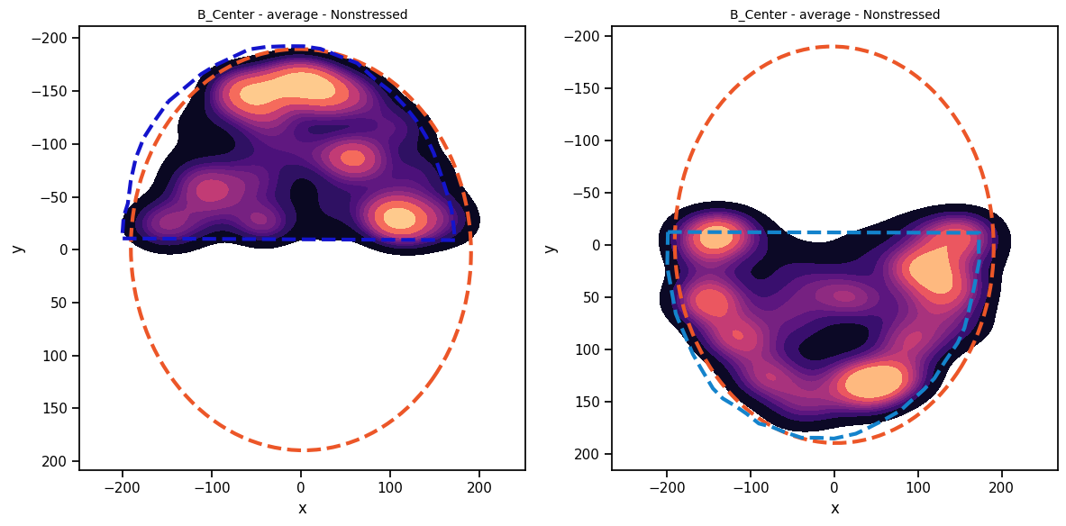
Furthermore, you can use regions of interest (ROIs) for spatial exploration, if you initialized them during project definition. Covering this here would be a bit much, so please have a look at the ROI tutorial for more details. For now, this is only a plot how ROIs in your data could look like:

# Load a previously saved project
my_deepof_project_with_rois = deepof.data.load_project("./tutorial_files/sample_project/")
# And load the experiment conditions
#my_deepof_project_with_rois.load_exp_conditions("./tutorial_files/tutorial_exp_conditions.csv")

# we now only plot

sns.set_context("notebook")

fig, (ax1, ax2) = plt.subplots(1, 2, figsize=(12, 6))

# Nose based plot
deepof.visuals.plot_heatmaps(
    my_deepof_project_with_rois,
    ["B_Center"],
    center="arena",
    exp_condition="CSDS",
    condition_value="Nonstressed",
    ax=ax1,
    show=False,
    display_arena=True,
    experiment_id="average",
    bin_index=2,
    bin_size=60,
    roi_number=1,
    animals_in_roi="B",
)

# Center based plot
deepof.visuals.plot_heatmaps(
    my_deepof_project_with_rois,
    ["B_Center"],
    center="arena",
    exp_condition="CSDS",
    condition_value="Nonstressed",
    ax=ax2,
    show=False,
    display_arena=True,
    experiment_id="average",
    bin_index=2,
    bin_size=60,
    roi_number=2,
    animals_in_roi="B",
)

plt.tight_layout()
plt.show()

Finally, let’s create an animated video showing our newly preprocessed data. DeepOF can produce reconstructions of the tracks and show them as videos. All animals and the arena are displayed by default. This is particularly useful when interpreting clusters and visualizing embeddings in the unsupervised pipeline, as we’ll see in a later turorial.

from IPython import display

video = deepof.visuals.animate_skeleton(
    my_deepof_project,
    experiment_id="20191204_Day2_SI_JB08_Test_54",
    bin_index=0,
    bin_size=20,
    sampling_rate=15,
    dpi=60,
)

html = display.HTML(video)
display.display(html)
plt.close()

What’s next

That’s it for this tutorial. Next, we’ll see how to run a supervised annotation pipeline with pretrained models!